07 Calculus: Multivariate
 Գյումրի, լուսանկարի հղումը, Հեղինակ՝ Naren Hakobyan
📚 Նյութը
YouTube links in this section were auto-extracted. If you spot a mistake, please let me know!
Դասախոսություն
Գործնական
🏡 Տնային
- ❗❗❗ DON’T CHECK THE SOLUTIONS BEFORE TRYING TO DO THE HOMEWORK BY YOURSELF❗❗❗
- Please don’t hesitate to ask questions, never forget about the 🍊karalyok🍊 principle!
- The harder the problem is, the more 🧀cheeses🧀 it has.
- Problems with 🎁 are just extra bonuses. It would be good to try to solve them, but also it’s not the highest priority task.
- If the problem involve many boring calculations, feel free to skip them - important part is understanding the concepts.
- Submit your solutions here (even if it’s unfinished)
01 Gradient Descent Algorithm
Consider the function \(f(x_1, x_2) = x_1^2 + 2x_2^2 + x_1 x_2 + 4x_1 - 2x_2 + 5\).
We want to find the minimum. We could do it analytically since it’s just a quadratic, but quite soon we’ll start to work with functions for which we can’t just find the optimum with pen and paper. So let’s use an iterative algorithm.
- Open up VS Code, or your favorite IDE.
- Pick a random starting point.
- In what direction should you move so that the function value decreases in the fastest way?
- Move in that direction. Consider multiplying the direction by a small value (say \(0.1\)) before taking the step. That multiplier is the learning rate \(\alpha\) (also called the step size), and it controls how aggressive each step is. Too big: you overshoot the optimum and diverge. Too small: convergence takes forever. The Armenian saying “ուշ ըլնի՝ նուշ ըլնի” (literally “let it be late, let it be almond”; loosely “better late and good than early and bad”) applies here.
- Keep iterating. Can you come up with a stopping criterion? (e.g., stop when the change in \(f\) between iterations falls below some threshold.)
- Plot and print interesting things, e.g., function value vs. iteration number.
- Play with \(\alpha\) and the starting point to see how convergence changes.
Expected outcome. With a sensible \(\alpha\) (try \(0.1\) first) the function value should decrease roughly monotonically and converge in a few dozen iterations. With \(\alpha\) too large you’ll see oscillation or blowup; with \(\alpha\) too small the loss will crawl downward and never quite finish.
02 Boat in Sevan
For a function \(f : \mathbb{R}^n \to \mathbb{R}\) and a unit vector \(\mathbf{u}\), the directional derivative of \(f\) at \(\mathbf{x}\) in direction \(\mathbf{u}\) is
\[D_{\mathbf{u}} f(\mathbf{x}) \;=\; \nabla f(\mathbf{x}) \cdot \mathbf{u}\]
It measures the instantaneous rate of change of \(f\) as you move from \(\mathbf{x}\) in direction \(\mathbf{u}\). Choosing \(\mathbf{u} = \mathbf{e}_i\) (the \(i\)-th standard basis vector) recovers the partial derivative \(\partial f / \partial x_i\).
Սևանա լճի \((x, y)\) կոորդինատներով կետում ջրի խորությունը
\[ f(x, y) = xy^2 - 6x^2 - 3y^2 \]
մետր է։ \((5, 3)\) կետում գտնվող «Նորատուս» առագաստանավի նավապետը ցանկանում է շարժվել դեպի մի այնպիսի կետ, որում ջուրն ավելի խոր է։ Նրա առաջին օգնականն առաջարկում է նավարկել դեպի հյուսիս, իսկ երկրորդը՝ դեպի հարավ։ Օգնականներից որի՞ խորհուրդը պետք է լսի նավապետը։
Setup. Depth at \((x, y)\) is \(f(x, y) = xy^2 - 6x^2 - 3y^2\). The captain stands at \((5, 3)\) and must decide between north (increasing \(y\), direction \((0, 1)\)) and south (decreasing \(y\), direction \((0, -1)\)).
The instantaneous rate of change of \(f\) when moving in a unit direction \(\mathbf{u}\) is the directional derivative:
\[D_{\mathbf{u}} f(\mathbf{x}) = \nabla f(\mathbf{x}) \cdot \mathbf{u}\]
So we just need \(\partial f / \partial y\) at \((5, 3)\), which is exactly the rate of change in the north direction.
Compute the gradient.
\[\frac{\partial f}{\partial x} = y^2 - 12x, \qquad \frac{\partial f}{\partial y} = 2xy - 6y\]
At \((5, 3)\):
\[\frac{\partial f}{\partial y}\bigg|_{(5,3)} = 2 \cdot 5 \cdot 3 - 6 \cdot 3 = 30 - 18 = 12 > 0\]
Decision. Moving north (direction \((0, 1)\)) gives directional derivative \(+12\): depth increases at a rate of \(12\) m per unit of distance. Moving south gives \(-12\): depth decreases. So the captain should listen to the first assistant and head north.
Sanity check on the full gradient. \(\nabla f(5, 3) = (9 - 60, \; 12) = (-51, 12)\). North isn’t actually the optimal direction; the steepest-ascent direction is \((-51, 12)/\|(-51, 12)\|\), roughly west-northwest. But between only the two options offered (north vs. south), north wins.
ML connection. This is exactly how gradient ascent works: project the gradient onto the available “moves” and pick the one with the highest dot product. In gradient descent we’d flip the sign and head in the direction with the most negative directional derivative.
03 Topless Box
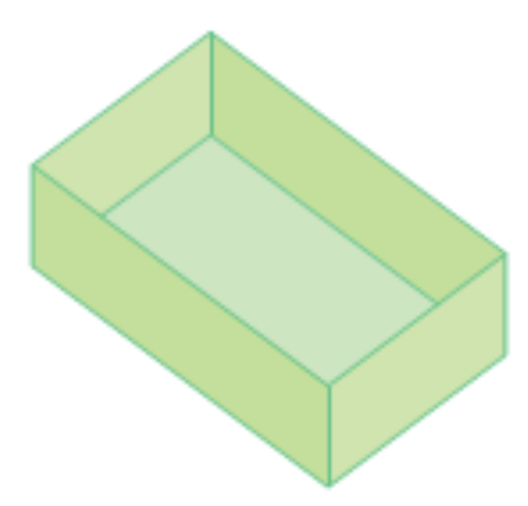
You have \(12\) m² of cardboard (plus scissors and glue) to build an open box (no top face). Unlike the earlier box problems, there are no square faces imposed here. What’s the maximum possible volume?
Hint: label the box’s three sides \(x\), \(y\), \(z\). Can you express \(z\) in terms of \(x\) and \(y\)? And then the volume?
Setup. Let the box have a rectangular base \(x \times y\) and height \(z\). With no top, there are 5 faces:
- bottom: area \(x y\)
- front & back: area \(2 x z\)
- left & right: area \(2 y z\)
Total surface area equals the budget: \[x y + 2 x z + 2 y z = 12\]
Solve for \(z\) (as the hint suggests): \[z = \frac{12 - x y}{2 (x + y)}\]
Volume to maximize: \[V(x, y) = x y z = \frac{x y (12 - x y)}{2 (x + y)}\]
Optimize. This is a genuine two-variable optimization: set \(\partial V / \partial x = 0\) and \(\partial V / \partial y = 0\). The problem is symmetric in \(x\) and \(y\) (swapping them changes neither the constraint nor the volume), so the interior optimum must satisfy \(x = y\). Substituting \(x = y\):
\[z = \frac{12 - x^2}{4 x}, \qquad V(x) = x^2 z = \frac{x (12 - x^2)}{4} = 3 x - \frac{x^3}{4}\]
\[V'(x) = 3 - \frac{3 x^2}{4} = 0 \;\Rightarrow\; x^2 = 4 \;\Rightarrow\; x = 2\]
Verify it’s a max. \(V''(x) = -\dfrac{3 x}{2}\), so \(V''(2) = -3 < 0\): local max. At the boundaries \(x \to 0\) and \(x \to \sqrt{12}\), \(V \to 0\), so this is the global max.
Plug back in. \(z = \dfrac{12 - 4}{8} = 1\), and \(y = x = 2\). The optimal box is \(2 \times 2 \times 1\) m: \[V_{\max} = 2 \cdot 2 \cdot 1 = 4 \text{ m}^3\]
The square base emerges on its own. We never required the base to be square, yet the optimum came out \(x = y = 2\). Just as the closed box turned out to be a cube (HW 05 Problem 01), the open box’s optimal base is a square. Symmetry keeps winning in these problems. The height \(z = 1\) is half the base side: with no top to pay for, the box spreads out lower and wider than a cube would.
04 Smooth Functions and Gradient Properties
A function \(f: \mathbb{R}^n \to \mathbb{R}\) is called smooth (or \(C^\infty\)) if it has continuous partial derivatives of all orders. In practice, we often work with \(C^1\) functions (continuously differentiable) or \(C^2\) functions (twice continuously differentiable).
Consider the bivariate function \(f : \mathbb{R}^2 \to \mathbb{R}\), \((x_1, x_2) \mapsto x_1^2 + 0.5x_2^2 + x_1x_2\).
- Show that \(f\) is smooth (continuously differentiable).
- Find the direction of greatest increase of \(f\) at \(\mathbf{x} = (1, 1)\).
- Find the direction of greatest decrease of \(f\) at \(\mathbf{x} = (1, 1)\).
- Find a direction in which \(f\) does not instantly change at \(\mathbf{x} = (1, 1)\).
- Assume there exists a differentiable parametrization of a curve \(\tilde{\mathbf{x}} : \mathbb{R} \to \mathbb{R}^2\), \(t \mapsto \tilde{\mathbf{x}}(t)\) such that \(\forall t \in \mathbb{R} : f(\tilde{\mathbf{x}}(t)) = f(1,1)\). Show that at each point of the curve \(\tilde{\mathbf{x}}\) the tangent vector \(\frac{\partial \tilde{\mathbf{x}}}{\partial t}\) is perpendicular to \(\nabla f(\tilde{\mathbf{x}})\).
- Interpret parts (d) and (e) geometrically.
\(f(x_1, x_2) = x_1^2 + 0.5 x_2^2 + x_1 x_2\).
1. Smoothness. \(f\) is a polynomial. All partial derivatives of all orders exist and are continuous everywhere (every derivative is itself a polynomial). So \(f \in C^\infty(\mathbb{R}^2)\), in particular \(C^1\). ✓
2. Direction of greatest increase at \((1, 1)\).
The gradient:
\[\nabla f(x_1, x_2) = \begin{pmatrix} 2x_1 + x_2 \\ x_2 + x_1 \end{pmatrix}\]
At \((1, 1)\): \(\nabla f(1, 1) = (3, 2)\).
The direction of greatest rate of increase is the unit gradient:
\[\mathbf{u}_{\uparrow} = \frac{\nabla f(1,1)}{\|\nabla f(1,1)\|} = \frac{1}{\sqrt{13}}\begin{pmatrix} 3 \\ 2 \end{pmatrix}\]
Why? For any unit vector \(\mathbf{u}\), \(D_{\mathbf{u}} f = \nabla f \cdot \mathbf{u} = \|\nabla f\|\cos\theta\), maximized when \(\theta = 0\), i.e., when \(\mathbf{u}\) is aligned with \(\nabla f\).
3. Direction of greatest decrease at \((1, 1)\).
By the same logic, \(D_{\mathbf{u}} f\) is minimized when \(\theta = \pi\), i.e., when \(\mathbf{u}\) is opposite to the gradient:
\[\mathbf{u}_{\downarrow} = -\frac{\nabla f(1,1)}{\|\nabla f(1,1)\|} = \frac{1}{\sqrt{13}}\begin{pmatrix} -3 \\ -2 \end{pmatrix}\]
This is exactly the direction gradient descent moves: “follow \(-\nabla f\).”
4. Direction of zero instantaneous change.
We need \(\nabla f(1, 1) \cdot \mathbf{u} = 0\), i.e. \(\mathbf{u}\) perpendicular to \((3, 2)\). Two unit choices:
\[\mathbf{u}_{\perp} = \pm \frac{1}{\sqrt{13}}\begin{pmatrix} -2 \\ 3 \end{pmatrix}\]
5. Tangent to a level curve is orthogonal to the gradient.
Suppose \(f(\tilde{\mathbf{x}}(t)) = c\) (constant) for all \(t\). Differentiate both sides with respect to \(t\) using the chain rule:
\[\frac{d}{dt} f(\tilde{\mathbf{x}}(t)) = \nabla f(\tilde{\mathbf{x}}(t)) \cdot \frac{d\tilde{\mathbf{x}}}{dt} = 0\]
Since the right-hand side is \(0\) for all \(t\), the tangent vector \(\frac{d\tilde{\mathbf{x}}}{dt}\) is perpendicular to \(\nabla f\) at every point of the curve. ✓
6. Geometric interpretation.
Part (4) found a direction where \(f\) doesn’t change instantaneously at \((1, 1)\). Part (5) showed that any curve along which \(f\) stays constant has its tangent perpendicular to \(\nabla f\). Together: the gradient is perpendicular to the level curves of \(f\).
This is one of the most important geometric facts in multivariate calculus:
- Level curves of \(f\) are the contour lines \(\{f = c\}\), like elevation lines on a topographic map.
- The gradient \(\nabla f\) points uphill, perpendicular to those contour lines, in the direction of steepest ascent.
- The directions you found in part (4) are tangents to the level curve passing through \((1, 1)\).
ML connection. Gradient descent moves perpendicular to the contour lines of the loss surface. This is why the trajectory zig-zags through long narrow valleys: each step is perpendicular to the current contour, but the contours of an ill-conditioned quadratic are stretched ellipses, so the perpendiculars don’t point at the minimum. Methods like Newton’s method and momentum fix this by not going strictly perpendicular to contours.
05 Contour Plots, Hessians, and Convexity
Contour plots (or level curves) visualize multivariate functions by showing curves where \(f(x_1, x_2) = c\) for various constants \(c\). They’re essential for understanding the shape of loss landscapes in machine learning.
Let \(f : \mathbb{R}^2 \to \mathbb{R}\), \((x_1, x_2) \mapsto -\cos(x_1^2 + x_2^2 + x_1x_2)\).
- Create a contour plot of \(f\) in the range \([-2,2] \times [-2,2]\) with R.
- Compute \(\nabla f\).
- Compute \(\nabla^2 f\) (the Hessian matrix).
Now, define the restriction of \(f\) to \(S_r = \{(x_1, x_2) \in \mathbb{R}^2 \mid x_1^2 + x_2^2 + x_1x_2 < r\}\) with \(r \in \mathbb{R}, r > 0\), i.e., \(f|_{S_r} : S_r \to \mathbb{R}, (x_1, x_2) \mapsto f(x_1, x_2)\).
- Show that \(f|_{S_r}\) with \(r = \pi/4\) is convex.
- Find the local minimum \(\mathbf{x}^*\) of \(f|_{S_r}\).
- Is \(\mathbf{x}^*\) a global minimum of \(f\)?
Let \(u(x_1, x_2) = x_1^2 + x_2^2 + x_1 x_2\) so \(f = -\cos(u)\). We’ll lean on the chain rule a lot; it’s much cleaner than expanding everything.
1. Contour plot (R skipped; we’ll just describe it).
The level sets \(\{f = c\}\) are determined by \(u(x_1, x_2) = \text{const}\). Since \(u\) is a positive-definite quadratic form (its matrix \(\bigl(\begin{smallmatrix} 1 & 1/2 \\ 1/2 & 1 \end{smallmatrix}\bigr)\) has eigenvalues \(\tfrac{3}{2}, \tfrac{1}{2}\), both positive), level sets of \(u\) are concentric ellipses centered at \((0, 0)\), with major axis along \((1, -1)\) and minor along \((1, 1)\). The contours of \(f = -\cos(u)\) are the same ellipses, but the function value oscillates as \(u\) grows: \(f = -1\) when \(u = 0, 2\pi, 4\pi, \ldots\) (deep blue rings) and \(f = +1\) when \(u = \pi, 3\pi, \ldots\) (red rings).
2. Gradient \(\nabla f\). By the chain rule, \(\nabla f = -\cos'(u) \cdot \nabla u = \sin(u) \nabla u\), where
\[\nabla u(x_1, x_2) = \begin{pmatrix} 2x_1 + x_2 \\ 2x_2 + x_1 \end{pmatrix}\]
So:
\[\nabla f(x_1, x_2) = \sin(x_1^2 + x_2^2 + x_1 x_2) \begin{pmatrix} 2x_1 + x_2 \\ 2x_2 + x_1 \end{pmatrix}\]
3. Hessian \(\nabla^2 f\). Differentiating \(\nabla f = \sin(u) \nabla u\) once more, by the product rule:
\[\nabla^2 f = \cos(u) \, (\nabla u)(\nabla u)^\top + \sin(u) \, \nabla^2 u\]
where \(\nabla^2 u = \bigl(\begin{smallmatrix} 2 & 1 \\ 1 & 2 \end{smallmatrix}\bigr)\) (constant) and \((\nabla u)(\nabla u)^\top\) is the rank-1 outer product:
\[(\nabla u)(\nabla u)^\top = \begin{pmatrix} (2x_1 + x_2)^2 & (2x_1+x_2)(2x_2+x_1) \\ (2x_1+x_2)(2x_2+x_1) & (2x_2 + x_1)^2 \end{pmatrix}\]
Combining:
\[\nabla^2 f = \cos(u)\,(\nabla u)(\nabla u)^\top + \sin(u)\begin{pmatrix} 2 & 1 \\ 1 & 2 \end{pmatrix}\]
4. Convexity on \(S_{\pi/4}\).
We need \(\nabla^2 f(\mathbf{x}) \succeq 0\) for all \(\mathbf{x} \in S_{\pi/4}\), i.e. all \(\mathbf{x}\) with \(0 \le u(\mathbf{x}) < \pi/4\).
- \(\cos(u) > 0\) on \(u \in [0, \pi/4)\) since \(\pi/4 < \pi/2\). ✓
- \((\nabla u)(\nabla u)^\top\) is rank-1 with eigenvalues \(\|\nabla u\|^2\) and \(0\): always positive semidefinite.
- \(\sin(u) > 0\) on \(u \in (0, \pi/4)\), and \(\nabla^2 u = \bigl(\begin{smallmatrix} 2 & 1 \\ 1 & 2 \end{smallmatrix}\bigr)\) has eigenvalues \(3, 1 > 0\): positive definite.
- At \(u = 0\) (i.e., at \(\mathbf{x} = 0\)), \(\sin(u) = 0\) and \(\nabla u = 0\), so \(\nabla^2 f = 0\) there: at least PSD.
A positive linear combination (with nonnegative scalars \(\cos(u), \sin(u)\)) of a PSD matrix and a PD matrix is PSD; on the open interior \(u \in (0, \pi/4)\) it’s actually PD. So \(f|_{S_{\pi/4}}\) is convex (and strictly convex on the interior except at the single point \(\mathbf{x} = 0\)).
5. Local minimum.
On \(S_{\pi/4}\), \(f\) is convex, so any stationary point is a global min of the restriction. From part 2, \(\nabla f = 0\) requires either \(\sin(u) = 0\) or \(\nabla u = 0\).
- \(\sin(u) = 0\) on \(S_{\pi/4}\) only at \(u = 0\) (since \(u \in [0, \pi/4)\)).
- \(\nabla u = (2x_1 + x_2, x_1 + 2x_2) = 0\) has unique solution \((x_1, x_2) = (0, 0)\), which gives \(u = 0\) anyway.
So \(\mathbf{x}^* = (0, 0)\) with \(f(\mathbf{x}^*) = -\cos(0) = -1\).
6. Is \(\mathbf{x}^*\) a global minimum of the full \(f\)?
Yes, because \(f(\mathbf{x}) = -\cos(u(\mathbf{x})) \ge -1\) for all \(\mathbf{x} \in \mathbb{R}^2\) (since \(\cos \le 1\)), and \(f(0, 0) = -1\). So \(-1\) is the global min, achieved at \(\mathbf{x}^* = (0, 0)\).
But it’s not the unique global min. \(f = -1\) whenever \(u = 2\pi k\) for any nonnegative integer \(k\), i.e., on every ellipse \(x_1^2 + x_2^2 + x_1 x_2 = 2\pi k\). So there are infinitely many points achieving the global minimum value, lying on a sequence of expanding ellipses around the origin.
ML connection. This is a great toy model of why convexity is local, not global, for many ML losses. Restricted to a small enough neighborhood, the loss surface looks convex and gradient descent finds the minimum cleanly. But globally, oscillating losses like this have many equivalent minima. Periodic activations and trigonometric reparameterizations (e.g. in Fourier features or sinusoidal positional encodings) inherit exactly this kind of geometry.
06 Taylor Expansion
Consider the bivariate function \(f : \mathbb{R}^2 \to \mathbb{R}, (x_1,x_2) \mapsto \exp(\pi \cdot x_1) - \sin(\pi \cdot x_2) + \pi \cdot x_1 \cdot x_2\).
- Compute the gradient of \(f\) for an arbitrary \(x\).
- Compute the Hessian of \(f\) for an arbitrary \(x\).
- State the first order taylor polynomial \(T_{1,a}(x)\) expanded around the point \(a = (0,1)\).
- State the second order taylor polynomial \(T_{2,a}(x)\) expanded around the point \(a = (0,1)\).
- Determine if \(T_{2,a}\) is a convex function.
\(f(x_1, x_2) = e^{\pi x_1} - \sin(\pi x_2) + \pi x_1 x_2\).
1. Gradient. Differentiate term by term:
\[\frac{\partial f}{\partial x_1} = \pi e^{\pi x_1} + \pi x_2, \qquad \frac{\partial f}{\partial x_2} = -\pi \cos(\pi x_2) + \pi x_1\]
\[\nabla f(x_1, x_2) = \pi \begin{pmatrix} e^{\pi x_1} + x_2 \\ -\cos(\pi x_2) + x_1 \end{pmatrix}\]
2. Hessian. Differentiate the gradient:
\[\frac{\partial^2 f}{\partial x_1^2} = \pi^2 e^{\pi x_1}, \quad \frac{\partial^2 f}{\partial x_2^2} = \pi^2 \sin(\pi x_2), \quad \frac{\partial^2 f}{\partial x_1 \partial x_2} = \pi\]
\[\nabla^2 f(x_1, x_2) = \begin{pmatrix} \pi^2 e^{\pi x_1} & \pi \\ \pi & \pi^2 \sin(\pi x_2) \end{pmatrix}\]
Evaluate at \(a = (0, 1)\):
- \(f(a) = e^0 - \sin(\pi) + \pi \cdot 0 \cdot 1 = 1 - 0 + 0 = 1\)
- \(\nabla f(a) = \pi \binom{1 + 1}{-\cos(\pi) + 0} = \pi \binom{2}{1}\) (using \(\cos\pi = -1\))
- \(\nabla^2 f(a) = \bigl(\begin{smallmatrix} \pi^2 & \pi \\ \pi & 0 \end{smallmatrix}\bigr)\) (using \(\sin\pi = 0\))
3. First-order Taylor polynomial around \(a\).
\[T_{1, a}(\mathbf{x}) = f(a) + \nabla f(a)^\top (\mathbf{x} - a) = 1 + \pi \begin{pmatrix} 2 \\ 1 \end{pmatrix}^\top \begin{pmatrix} x_1 \\ x_2 - 1 \end{pmatrix}\]
\[\boxed{\;T_{1, a}(\mathbf{x}) = 1 + 2\pi x_1 + \pi(x_2 - 1)\;}\]
4. Second-order Taylor polynomial around \(a\).
\[T_{2, a}(\mathbf{x}) = T_{1, a}(\mathbf{x}) + \tfrac{1}{2}(\mathbf{x} - a)^\top \nabla^2 f(a) (\mathbf{x} - a)\]
Compute the quadratic term with \(\mathbf{x} - a = (x_1, \, x_2 - 1)^\top\):
\[\tfrac{1}{2}(x_1, \; x_2 - 1) \begin{pmatrix} \pi^2 & \pi \\ \pi & 0 \end{pmatrix} \begin{pmatrix} x_1 \\ x_2 - 1 \end{pmatrix} = \tfrac{1}{2}\Big[\pi^2 x_1^2 + 2\pi x_1(x_2 - 1)\Big]\]
\[= \tfrac{\pi^2}{2} x_1^2 + \pi x_1 (x_2 - 1)\]
So:
\[\boxed{\;T_{2, a}(\mathbf{x}) = 1 + 2\pi x_1 + \pi(x_2 - 1) + \tfrac{\pi^2}{2} x_1^2 + \pi x_1 (x_2 - 1)\;}\]
5. Is \(T_{2, a}\) convex?
A quadratic is convex iff its Hessian is positive semidefinite. The Hessian of \(T_{2, a}\) is exactly \(\nabla^2 f(a) = \bigl(\begin{smallmatrix} \pi^2 & \pi \\ \pi & 0 \end{smallmatrix}\bigr)\).
Check via determinant + trace:
- \(\det = \pi^2 \cdot 0 - \pi \cdot \pi = -\pi^2 < 0\)
- Trace \(= \pi^2 > 0\)
Since \(\det < 0\), the eigenvalues have opposite signs (one positive, one negative). The Hessian is indefinite → \(T_{2, a}\) is neither convex nor concave. It’s a saddle-shaped quadratic.
Why the second-order Taylor can be non-convex. A common misconception is that the second-order Taylor expansion is always a “bowl.” That’s only true if the original function has a positive-definite Hessian at the expansion point. Here, \(f\) is not convex globally, and at the point \((0, 1)\) specifically, \(\sin(\pi \cdot 1) = 0\) kills the \(\partial^2 / \partial x_2^2\) entry, leaving the Hessian indefinite.
ML connection. Newton’s method approximates the loss locally by its second-order Taylor expansion and then jumps to that quadratic’s minimum. But if the local Hessian is indefinite (we’re near a saddle, not a basin), Newton’s method can step toward the saddle instead of away. This is a real failure mode in deep-learning loss landscapes, which are full of saddles. Modifications like trust-region and saddle-free Newton address it by replacing \(H\) with \(|H|\) (taking absolute values of eigenvalues).
Problems from the Armenian notes (Section 7.7)
These problems are extracted from Section 7.7 of the Armenian course notes (PDF page 97). The Boat in Sevan (notes 7.7 #4) and the topless box (notes 7.7 #7) already appear above as problems 02 and 03; the five below are the rest of the set.
07 Match Functions to Graphs (notes 7.7 #1)
Match each function to its graph:
- \(f(x,y) = |x| + |y|\)
- \(f(x,y) = |xy|\)
- \(f(x,y) = \dfrac{1}{1 + x^2 + y^2}\)
- \(f(x,y) = (x^2 - y^2)^2\)
- \(f(x,y) = (x - y)^2\)
- \(f(x,y) = \sin(|x| + |y|)\)
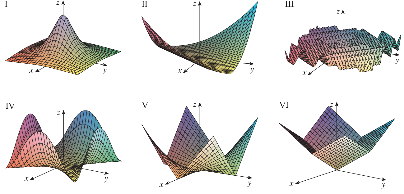
| Function | Graph | Distinguishing feature |
|---|---|---|
| a. \(\lvert x\rvert + \lvert y\rvert\) | VI | Pyramid-shaped valley: flat triangular faces, linear rise from the origin, diamond-shaped level sets (the \(\ell_1\) norm). |
| b. \(\lvert xy\rvert\) | V | Zero along both axes (sharp creases there), rising to four peaks in the diagonal directions. Sharp ridges signal the absolute value. |
| c. \(\dfrac{1}{1+x^2+y^2}\) | I | A single smooth bump: maximum \(1\) at the origin, decaying radially to \(0\). The only bounded, everywhere-positive surface. |
| d. \((x^2 - y^2)^2\) | IV | Smooth (polynomial), zero along both diagonals \(y = \pm x\), rising to humps along the axes. Four-fold structure with valleys on the diagonals. |
| e. \((x - y)^2\) | II | A smooth parabolic trough: zero along the line \(y = x\), rising quadratically perpendicular to it. A U extruded along one diagonal. |
| f. \(\sin(\lvert x\rvert + \lvert y\rvert)\) | III | Oscillating concentric diamond ripples, since the wavefronts \(\lvert x\rvert + \lvert y\rvert = \text{const}\) are diamonds. The only periodic surface. |
How to tell them apart quickly. Three cues do most of the work:
- Where is the function zero? On the axes → \(\lvert xy\rvert\) (V). On the diagonals → \((x^2-y^2)^2\) (IV) and \((x-y)^2\) (II, zero only on \(y=x\)).
- Smooth or creased? Absolute values and the \(\ell_1\) norm produce sharp creases (V, VI); polynomials are smooth (II, IV).
- Bounded, bumpy, or periodic? Only \(\frac{1}{1+x^2+y^2}\) is a single bounded bump (I); only \(\sin(\cdot)\) oscillates (III).
08 Partial Derivatives (notes 7.7 #2)
Find the partial derivatives \(\partial f/\partial x\) and \(\partial f/\partial y\):
- \(f(x,y) = 3x - 2y^2\)
- \(f(x,y) = y^7 - 2x^3 + x^2\)
- \(f(x,y) = \sin(xy)\)
- \(f(x,y) = x \ln y + \dfrac{x}{y}\)
The rule: to differentiate with respect to one variable, treat the other variable as a constant.
a. \(\dfrac{\partial f}{\partial x} = 3, \qquad \dfrac{\partial f}{\partial y} = -4y\)
b. \(\dfrac{\partial f}{\partial x} = -6x^2 + 2x, \qquad \dfrac{\partial f}{\partial y} = 7y^6\)
c. Chain rule, holding the other variable fixed: \[\dfrac{\partial f}{\partial x} = y\cos(xy), \qquad \dfrac{\partial f}{\partial y} = x\cos(xy)\]
d. With \(x\) as a constant multiplier for the \(x\)-derivative, and using \((\ln y)' = 1/y\) plus \((x/y)' = -x/y^2\) for the \(y\)-derivative: \[\dfrac{\partial f}{\partial x} = \ln y + \dfrac{1}{y}, \qquad \dfrac{\partial f}{\partial y} = \dfrac{x}{y} - \dfrac{x}{y^2} = \dfrac{x(y-1)}{y^2}\]
09 Directional Derivatives (notes 7.7 #3)
Compute the directional derivative along \(\mathbf{v} = \begin{bmatrix} 0.6 & 0.8 \end{bmatrix}\) at the point \((-1, -1)\):
- \(f(x,y) = 3xy\)
- \(f(x,y) = 1 - x^2\)
- \(f(x,y) = e^{x-y}\)
First check that \(\mathbf{v}\) is a unit vector (otherwise the directional derivative formula needs normalizing): \(0.6^2 + 0.8^2 = 0.36 + 0.64 = 1\). ✓ Good, it’s the familiar 3-4-5 direction.
Then \(D_{\mathbf{v}} f = \nabla f \cdot \mathbf{v}\), evaluated at \((-1,-1)\).
a. \(\nabla f = (3y, 3x)\), so \(\nabla f(-1,-1) = (-3, -3)\): \[D_{\mathbf{v}} f = (-3)(0.6) + (-3)(0.8) = -1.8 - 2.4 = -4.2\]
b. \(\nabla f = (-2x, 0)\), so \(\nabla f(-1,-1) = (2, 0)\): \[D_{\mathbf{v}} f = (2)(0.6) + (0)(0.8) = 1.2\]
c. \(\nabla f = (e^{x-y}, -e^{x-y})\). At \((-1,-1)\), \(x - y = 0\) so \(e^0 = 1\), giving \(\nabla f = (1, -1)\): \[D_{\mathbf{v}} f = (1)(0.6) + (-1)(0.8) = -0.2\]
Reading the signs. In direction \(\mathbf{v}\), function (a) decreases steeply, (b) increases, and (c) decreases slightly. The directional derivative is just the gradient’s “shadow” on \(\mathbf{v}\): how much of the gradient points along your chosen direction.
10 Local Extrema (notes 7.7 #5)
Find the local minima and maxima (if any):
- \(f(x,y) = 3xy\)
- \(f(x,y) = x^2 - xy\)
- \(f(x,y) = 2x^2 - x^3 - y^2\)
- \(f(x,y) = x^3 - 3x - y^3 + 3y\)
The recipe: find critical points (\(\nabla f = 0\)), then classify each with the Hessian \(H\). For a \(2\times2\) Hessian, the second-derivative test reads:
- \(\det H > 0\) and \(\operatorname{tr} H > 0\) → local min
- \(\det H > 0\) and \(\operatorname{tr} H < 0\) → local max
- \(\det H < 0\) → saddle (no extremum)
a. \(\nabla f = (3y, 3x) = 0 \Rightarrow (0,0)\). Hessian \(\bigl(\begin{smallmatrix} 0 & 3 \\ 3 & 0 \end{smallmatrix}\bigr)\), \(\det = -9 < 0\): saddle. No extrema.
b. \(\nabla f = (2x - y, -x) = 0 \Rightarrow (0,0)\). Hessian \(\bigl(\begin{smallmatrix} 2 & -1 \\ -1 & 0 \end{smallmatrix}\bigr)\), \(\det = -1 < 0\): saddle. No extrema.
c. \(\nabla f = (4x - 3x^2, -2y) = 0\). Second equation gives \(y = 0\); first gives \(x(4 - 3x) = 0\), so \(x = 0\) or \(x = 4/3\). Hessian \(\bigl(\begin{smallmatrix} 4 - 6x & 0 \\ 0 & -2 \end{smallmatrix}\bigr)\).
- \((0, 0)\): \(\det = (4)(-2) = -8 < 0\): saddle.
- \((4/3, 0)\): \(4 - 6 \cdot \tfrac{4}{3} = -4\), so \(\det = (-4)(-2) = 8 > 0\), \(\operatorname{tr} = -6 < 0\): local max, value \(f(4/3, 0) = \tfrac{32}{27}\).
d. \(\nabla f = (3x^2 - 3, -3y^2 + 3) = 0 \Rightarrow x = \pm 1, \; y = \pm 1\): four critical points. Hessian \(\bigl(\begin{smallmatrix} 6x & 0 \\ 0 & -6y \end{smallmatrix}\bigr)\).
| Point | \(\det H\) | \(\operatorname{tr} H\) | Type | \(f\) |
|---|---|---|---|---|
| \((1, 1)\) | \(-36\) | \(0\) | saddle | \(0\) |
| \((1, -1)\) | \(36\) | \(12\) | local min | \(-4\) |
| \((-1, 1)\) | \(36\) | \(-12\) | local max | \(4\) |
| \((-1, -1)\) | \(-36\) | \(0\) | saddle | \(0\) |
Takeaway. A zero gradient is necessary but not sufficient: of the 8 critical points across these four functions, most are saddles. In high dimensions saddles vastly outnumber true minima, which is exactly why naive Newton’s method struggles on neural-net loss surfaces (see problem 06).
11 TV Tower Placement (notes 7.7 #6)
A TV tower must be built to serve four villages at \((-5, 0)\), \((1, 7)\), \((9, 0)\), and \((0, -8)\). At which point \((x, y)\) should the tower go so that the sum of squared distances from the villages is as small as possible?
Hint: plot the points and write each one’s distance from \((x, y)\). What is the sum of their squares?
Let the four villages be \((a_i, b_i)\). Minimize: \[S(x, y) = \sum_{i=1}^{4} \big[(x - a_i)^2 + (y - b_i)^2\big]\]
Set the partials to zero: \[\frac{\partial S}{\partial x} = \sum_i 2(x - a_i) = 0 \;\Rightarrow\; 4x = \sum_i a_i \;\Rightarrow\; x = \bar a\] \[\frac{\partial S}{\partial y} = \sum_i 2(y - b_i) = 0 \;\Rightarrow\; 4y = \sum_i b_i \;\Rightarrow\; y = \bar b\]
So the optimum is the centroid (the average of the points): \[x = \frac{-5 + 1 + 9 + 0}{4} = \frac{5}{4} = 1.25, \qquad y = \frac{0 + 7 + 0 - 8}{4} = -\frac{1}{4} = -0.25\]
The Hessian is \(\bigl(\begin{smallmatrix} 8 & 0 \\ 0 & 8 \end{smallmatrix}\bigr)\), positive definite, so \((1.25, -0.25)\) is indeed the minimizer.
Why this is a big deal. The point minimizing the sum of squared distances is always the plain average of the coordinates. This is the 2D version of the single most-used fact in statistics and ML: the mean is the least-squares estimator. It’s why linear regression minimizes squared error (the fitted values land at conditional means), why k-means uses centroids as cluster centers, and why the “average” is the default summary of data. Note it would be a different point if we minimized the sum of un-squared distances (that gives the geometric median, which has no closed form). Squaring is what makes the answer clean.