29: Information Theory - Entropy, Cross-Entropy, KL Divergence
📚 Նյութը
Դասախոսություն
- 📺 Դասախոսություն — Entropy, Source Coding, Cross-Entropy, KL
- 📺 Գործնական — Information Theory practical
- 🎞️ Սլայդեր — info 01, 📝 Notes
- 🐍 Գործնականի notebook
- 🛠️🗂️ Գործնականի PDF-ը
This practical covers info_01 only: entropy, surprisal, source coding, cross-entropy, KL divergence, and differential entropy. Mutual information, MLE, and MaxEnt come in the next lecture (info_02).
🏡 Տնային
01 ✏️🐍 Armenian Alphabet Entropy
The Armenian alphabet has 39 letters (Mashtots’ original 36 + ՈՒ, Օ, Ֆ).
a) Compute the uniform entropy: how many bits per letter if every letter were equally likely?
b) English’s uniform bound is \(\log_2 26 \approx 4.70\) bits/letter, yet real English text has empirical entropy around \(1.3\) bits/letter (Shannon, 1951). Explain why the empirical entropy is so much smaller than the uniform bound. Name the two distinct effects.
c) (Python) Estimate the real per-letter entropy of Armenian. Use the provided file assets/panir_hy.txt (the «Պանիր» Wikipedia article), or download fresh text yourself with the snippet below. Keep only Armenian letters, lowercase them, and compute the empirical letter-frequency distribution and its entropy.
# Option A — download the provided text file:
import urllib.request
url = ("https://raw.githubusercontent.com/HaykTarkhanyan/"
       "python_math_ml_course/main/math/assets/panir_hy.txt")
text = urllib.request.urlopen(url).read().decode("utf-8")

# Option B — download any Armenian article's plain text yourself:
import urllib.request, urllib.parse, json
title = "Պանիր"  # try any article title
url = "https://hy.wikipedia.org/w/api.php?" + urllib.parse.urlencode({
    "action": "query", "prop": "extracts", "explaintext": 1,
    "titles": title, "format": "json", "redirects": 1,
})
req = urllib.request.Request(url, headers={"User-Agent": "course/1.0"})
page = next(iter(json.load(urllib.request.urlopen(req))["query"]["pages"].values()))
text = page["extract"]
d) Compare your empirical entropy to the uniform bound from (a). By roughly how many bits per letter does the frequency skew save you?
e) A 100-page Armenian e-book has roughly \(200{,}000\) characters. Estimate the entropy lower bound on its size (KB). Then explain the catch: you’ll get \(\approx 4.5\) bits/letter, but a real code must assign a whole number of bits to each letter — so how do you actually get close to the entropy?
(a) A uniform distribution over \(g\) outcomes has entropy \(\log_2 g\). So \[H_{\text{uniform}} = \log_2 39 \approx 5.29 \text{ bits/letter}.\] This is the maximum possible per-letter entropy for a 39-letter alphabet.
(b) Two separate effects pull the real entropy below the uniform bound:
- Non-uniform letter frequencies. Entropy is maximized only by the uniform distribution; any skew lowers it. Common letters (ա, ե, ի, ն, ո) appear far more than rare ones, so each letter carries less than the maximal \(5.29\) bits.
- Inter-letter correlations. Real text is not i.i.d. — after «ա» some letters are much likelier than others. Modeling context (letter pairs, words) reduces the per-letter entropy much further. The \(1.3\) bits/letter figure for English uses this contextual structure.
(c) Full implementation. The one subtlety is filtering to the Armenian Unicode block, or Latin letters from foreign words and references inflate the alphabet to 70+ “letters”:
from collections import Counter
import math, urllib.request

url = ("https://raw.githubusercontent.com/HaykTarkhanyan/"
       "python_math_ml_course/main/math/assets/panir_hy.txt")
text = urllib.request.urlopen(url).read().decode("utf-8")

def is_armenian(ch):  # U+0531–U+0556 upper, U+0561–U+0587 lower
    o = ord(ch)
    return 0x0531 <= o <= 0x0556 or 0x0561 <= o <= 0x0587

letters = [c for c in text.lower() if is_armenian(c)]
counts = Counter(letters)
n = len(letters)
H = -sum((c / n) * math.log2(c / n) for c in counts.values())
print(f"{n} letters, {len(counts)} distinct")
print(f"empirical entropy = {H:.3f} bits/letter")
Output on the provided file:
22417 letters, 39 distinct
empirical entropy = 4.484 bits/letter
(d) Empirical \(4.48\) vs uniform \(5.29\) ⇒ the frequency skew saves about \(\mathbf{0.8}\) bits/letter. The single most common letter «ա» is already ~15% of all letters. (Contextual modeling would save far more.)
(e) Naive entropy lower bound: \[200{,}000 \times 4.48 \text{ bits} = 896{,}000 \text{ bits} \approx \mathbf{109 \text{ KB}}.\]
The discrete catch. Entropy is \(4.48\) bits/letter, but a real prefix code assigns an integer number of bits per symbol — you can’t literally spend \(4.48\) bits on one letter. So:
- A fixed-length code needs \(\lceil\log_2 39\rceil = \mathbf{6}\) bits/letter ⇒ \(200{,}000 \times 6 / 8 / 1024 \approx 146\) KB. Easy, but wastes \(6 - 4.48 = 1.5\) bits/letter.
- A Huffman code on single letters does better (frequent letters get short codewords), landing between \(H\) and \(H + 1\).
- To actually approach \(4.48\) you must encode blocks of several letters at once (or use arithmetic coding). The source coding theorem is asymptotic: expected bits/symbol \(\to H\) only as block length grows. So \(4.48\) is the theoretical floor — an average you approach with block coding, not a per-letter code length you can use directly.
02 🐍 Wordle as an Information Game
We may skip this one during the practical (it’s a bigger coding task) — it’s here for you to enjoy on your own.
Wordle has \(N = 2{,}315\) valid answer words. Each guess comes back as a color pattern: every one of the 5 letters is green (right letter, right spot), yellow (right letter, wrong spot), or gray (not in the word). With 3 colors on 5 positions there are \(3^5 = 243\) possible patterns.
Grab the official answer list (2,315 words) like this:
import urllib.request
url = ("https://gist.githubusercontent.com/cfreshman/"
       "a03ef2cba789d8cf00c08f767e0fad7b/raw/wordle-answers-alphabetical.txt")
words = urllib.request.urlopen(url).read().decode().split()
assert len(words) == 2315
a) Think of a guess as a question whose answer is the color pattern. At most how many distinct answers can that question have — and therefore how many bits can one guess reveal at most?
b) How many bits of uncertainty does the answer carry before any guess? Combining (a) and (b), what’s the minimum number of guesses an ideal solver would need in the best case?
c) Implement a greedy solver: for each candidate guess \(g\), partition the current answer set by their color pattern against \(g\), and compute the entropy of that partition. Pick the \(g\) with the highest entropy (it splits the candidates most evenly).
from collections import Counter
import math

def feedback(guess: str, answer: str) -> tuple:
    """Color pattern as a 5-tuple of 'G' (green), 'Y' (yellow), '.' (gray).
    Careful: a letter appearing once in the answer but twice in the guess
    earns only one Y/G total."""
    ...

def expected_info(guess, candidates):
    counts = Counter(feedback(guess, a) for a in candidates)
    n = len(candidates)
    return -sum((c/n) * math.log2(c/n) for c in counts.values())
d) Report the top-5 first guesses your solver finds and their entropies in bits. Compare to popular openers (CRANE, SLATE, RAISE).
e) Explain in entropy terms why the solver never recommends a word like FUZZY or AAHED as a first guess.
f) (Bardle — Armenian Wordle.) The same game exists in Armenian: Bardle. Re-run your exact solver on the Armenian 5-letter answer set assets/bardle_hy_5_answers.txt (178 words); the allowed-guess list is assets/bardle_hy_5_guesses.txt (2,855 words). Then answer:
- How much starting uncertainty (bits) does the 178-word answer set carry, vs English Wordle’s 2,315?
- Is the per-guess ceiling still \(\log_2 243\)? Why or why not — does Armenian’s 39-letter alphabet change it?
- Report the top-3 Armenian opening guesses your solver finds.
(a) What \(\log_2 243\) represents. A guess does not return a word — it returns one of the 243 possible color patterns. So a guess behaves like a question with up to 243 possible answers. Any question is most informative when all its answers are equally likely; then the answer carries \[\log_2(\text{number of possible answers}) = \log_2 243 \approx 7.92 \text{ bits}.\] That is the ceiling: no single guess can ever reveal more than \(7.92\) bits, because there are only 243 distinguishable responses to read. (Real guesses reveal less — many of the 243 patterns almost never occur, so they are far from equally likely.)
(b) Before guessing, the hidden word is roughly uniform over 2,315 words, so the starting uncertainty is \[H = \log_2 2315 \approx 11.18 \text{ bits}.\] If every guess delivered the full \(7.92\) bits you’d need \(\lceil 11.18 / 7.92 \rceil = 2\) guesses. In reality a guess reveals only \(\sim 5\)–\(6\) bits, so the proven optimum averages about \(3.42\) guesses (Selby, 2022).
A worked turn. Suppose the hidden word is ROBIN and you open with SLATE:
| Letter | In ROBIN? | Color |
|---|---|---|
| S | no | gray . |
| L | no | gray . |
| A | no | gray . |
| T | no | gray . |
| E | no | gray . |
The pattern is ..... (all gray). Every answer that contains none of S, L, A, T, E returns this same pattern — still hundreds of words — so this particular turn revealed only a few bits. You now keep only answers consistent with “no S, L, A, T, E” and pick the next max-entropy guess. A sharper guess like CRANE against ROBIN returns a pattern with R and N yellow, which slices the candidate set far more.
(c) Full implementation (the greens-before-yellows order with a letter pool is the only tricky part):
from collections import Counter
import math

def feedback(guess, answer):
    res = ['.'] * 5
    pool = Counter(answer)
    for i in range(5):                       # greens first
        if guess[i] == answer[i]:
            res[i] = 'G'; pool[guess[i]] -= 1
    for i in range(5):                       # then yellows from what's left
        if res[i] == '.' and pool[guess[i]] > 0:
            res[i] = 'Y'; pool[guess[i]] -= 1
    return tuple(res)

def expected_info(guess, candidates):
    counts = Counter(feedback(guess, a) for a in candidates)
    n = len(candidates)
    return -sum((c / n) * math.log2(c / n) for c in counts.values())

best = sorted(words, key=lambda g: expected_info(g, words), reverse=True)[:5]
for g in best:
    print(g.upper(), round(expected_info(g, words), 2), "bits")
(d) This prints top openers like SALET, REAST, CRATE, TRACE, SLATE, each \(\approx 5.8\)–\(5.9\) bits. Human favorites (CRANE, RAISE) score nearly as high — that is why they are good: they split the answer set evenly.
(e) FUZZY has a repeated Z and rare letters. Most answers contain none of F, U, Z, Y, so they all return the same all-gray pattern — the 2,315 words collapse into a few big buckets. Few buckets ⇒ low partition entropy ⇒ little information. Good openers use 5 distinct, common letters to spread answers across many buckets.
(f) The color-pattern logic is identical (5 positions, 3 colors), so the same feedback/expected_info code runs unchanged on Armenian strings — it indexes characters generically:
ans = open("assets/bardle_hy_5_answers.txt", encoding="utf-8").read().split()
guesses = open("assets/bardle_hy_5_guesses.txt", encoding="utf-8").read().split()
best = sorted(guesses, key=lambda g: expected_info(g, ans), reverse=True)[:3]- Starting uncertainty: \(\log_2 178 \approx \mathbf{7.48}\) bits — far less than English Wordle’s \(\log_2 2315 \approx 11.18\), because Bardle’s curated answer set is much smaller.
- The per-guess ceiling is still \(\log_2 243 \approx 7.92\) bits. It depends only on the number of distinguishable responses (\(3^5\) patterns from 5 positions × 3 colors), not on the alphabet size — Armenian’s 39 letters do not change it. (Notably, the starting uncertainty \(7.48\) is below the single-guess ceiling, so a perfect opener could in principle pin most answers in just one or two guesses.)
- Top-3 openers: կարեն (5.34 bits), նոտար (5.30), կարին (5.25). Fittingly, «Կարեն» — one of the most common Armenian names — is the single best opening guess.
03 ✏️ Source Coding: Huffman & the Kraft Inequality (Optional)
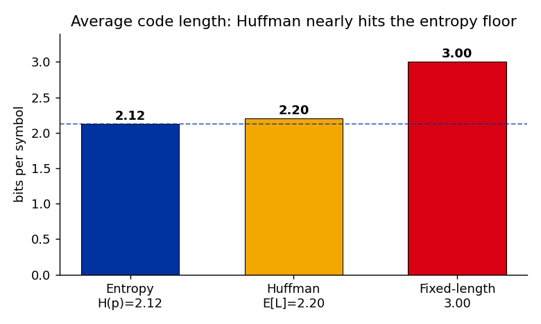
A source emits 5 symbols with probabilities \[p = (\,A{:}\,0.4,\; B{:}\,0.2,\; C{:}\,0.2,\; D{:}\,0.1,\; E{:}\,0.1\,).\]
a) Compute the entropy \(H(p)\) in bits.
b) Build a Huffman code: repeatedly merge the two least-probable nodes. Draw the final tree and list each codeword and its length.
c) Compute the expected code length \(\mathbb{E}[L] = \sum_i p_i L_i\). Verify Shannon’s bound \(H(p) \le \mathbb{E}[L] < H(p) + 1\).
d) Verify your code satisfies the Kraft inequality \(\sum_i 2^{-L_i} \le 1\). Is it saturated (equal to 1)? Why does that make sense for a Huffman code?
e) A naive fixed-length code needs \(\lceil \log_2 5 \rceil = 3\) bits per symbol. How many bits per symbol does Huffman save on average?
(a) Plug into \(H = -\sum_i p_i \log_2 p_i\). Useful values: \(\log_2 0.4 = -1.322\), \(\log_2 0.2 = -2.322\), \(\log_2 0.1 = -3.322\). \[H(p) = -\big(0.4(-1.322) + 2\cdot 0.2(-2.322) + 2\cdot 0.1(-3.322)\big) = 0.529 + 0.929 + 0.664 = \mathbf{2.12 \text{ bits}}.\]
(b) Huffman repeatedly merges the two least-probable nodes; the merged node’s probability is their sum. Track it step by step:
| Step | Pool (prob) | Merge | New node |
|---|---|---|---|
| 1 | A·4, B·2, C·2, D·1, E·1 | D+E | DE = 0.2 |
| 2 | A·4, B·2, C·2, DE·2 | B+C | BC = 0.4 |
| 3 | A·4, DE·2, BC·4 | DE+A | ADE = 0.6 |
| 4 | BC·4, ADE·6 | BC+ADE | root = 1.0 |
(probabilities written ×10 for readability). Reading the tree from the root, assigning 0 to the left branch and 1 to the right:
              root
          0 /      \ 1
          BC        ADE
        0/  \1     0/   \1
        B    C     A     DE
                       0/   \1
D E| Symbol | \(p\) | Codeword | Length \(L_i\) | Surprisal \(-\log_2 p_i\) |
|---|---|---|---|---|
| A | 0.4 | 10 |
2 | 1.32 |
| B | 0.2 | 00 |
2 | 2.32 |
| C | 0.2 | 01 |
2 | 2.32 |
| D | 0.1 | 110 |
3 | 3.32 |
| E | 0.1 | 111 |
3 | 3.32 |
Notice each length \(L_i\) sits right next to the surprisal \(-\log_2 p_i\) — Huffman approximates the ideal \(L_i = -\log_2 p_i\) using whole bits. (Tie-breaking can give a different but equally good tree.)
(c) \[\mathbb{E}[L] = 0.4(2) + 0.2(2) + 0.2(2) + 0.1(3) + 0.1(3) = \mathbf{2.2 \text{ bits}}.\] Shannon’s bound holds: \(2.12 \le 2.2 < 3.12\). ✓ Efficiency \(H/\mathbb{E}[L] = 2.12/2.2 \approx 0.96\).
(d) \[\sum_i 2^{-L_i} = \underbrace{3\cdot 2^{-2}}_{A,B,C} + \underbrace{2\cdot 2^{-3}}_{D,E} = \tfrac{3}{4} + \tfrac{1}{4} = 1.\] Saturated (\(=1\)). A Huffman tree has no unused leaves, so there’s no spare bit-budget — the same “no room for a 5th codeword” idea from the lecture’s Kraft slide.
(e) Fixed-length costs \(\lceil\log_2 5\rceil = 3\) bits/symbol; Huffman costs \(2.2\). Saving \(3 - 2.2 = \mathbf{0.8}\) bits/symbol (\(\sim 27\%\)), landing just above the \(2.12\)-bit entropy floor:
04 ✏️ Cross-Entropy and KL: The Cost of the Wrong Code
The true distribution of a 4-symbol source is \(p = (\tfrac{1}{2}, \tfrac{1}{4}, \tfrac{1}{8}, \tfrac{1}{8})\). A lazy engineer assumes it’s uniform, \(q = (\tfrac{1}{4}, \tfrac{1}{4}, \tfrac{1}{4}, \tfrac{1}{4})\), and builds the optimal code for \(q\) (i.e. a fixed-length 2-bit code).
a) Compute \(H(p)\) and \(H(q)\).
b) Compute the cross-entropy \(H(p \| q) = -\sum_x p(x)\log_2 q(x)\) — the average code length when the data really comes from \(p\) but we use \(q\)’s code.
c) Compute \(D_{\text{KL}}(p \| q)\) and verify the identity \(H(p\|q) = H(p) + D_{\text{KL}}(p\|q)\).
d) In one sentence: how many bits per symbol does the engineer waste by using the uniform (fixed-length) code instead of the optimal one for \(p\)?
e) Is \(D_{\text{KL}}\) symmetric? State whether \(D_{\text{KL}}(p\|q) = D_{\text{KL}}(q\|p)\) holds in general (you don’t need to recompute — just recall the lecture).
(a) \[H(p) = \tfrac{1}{2}(1) + \tfrac{1}{4}(2) + \tfrac{1}{8}(3) + \tfrac{1}{8}(3) = \mathbf{1.75 \text{ bits}}, \qquad H(q) = \log_2 4 = \mathbf{2 \text{ bits}}.\]
(b) Since \(q(x) = \tfrac14\) for all \(x\), \(\log_2 q(x) = -2\), so \[H(p\|q) = -\sum_x p(x)(-2) = 2\sum_x p(x) = \mathbf{2 \text{ bits}}.\] (Makes sense: \(q\)’s optimal code is the fixed-length 2-bit code, so every symbol costs 2 bits.)
(c) \[D_{\text{KL}}(p\|q) = \sum_x p(x)\log_2\tfrac{p(x)}{q(x)} = \tfrac12\log_2 2 + \tfrac14\log_2 1 + 2\cdot\tfrac18\log_2\tfrac12 = \tfrac12 - \tfrac14 = \mathbf{0.25 \text{ bits}}.\] Identity check: \(H(p) + D_{\text{KL}}(p\|q) = 1.75 + 0.25 = 2 = H(p\|q)\). ✓
(d) The engineer wastes exactly \(D_{\text{KL}}(p\|q) = \mathbf{0.25}\) bits per symbol — the gap between the \(2\)-bit wrong code and the \(1.75\)-bit optimal code.
(e) No — \(D_{\text{KL}}\) is not symmetric in general: \(D_{\text{KL}}(p\|q) \ne D_{\text{KL}}(q\|p)\) for most pairs. It is a divergence, not a distance. (This particular \(p\)/uniform-\(q\) pair is a special case where the two happen to coincide, but don’t be fooled — it fails as soon as \(q\) is non-uniform.)
05 ✏️ Differential Entropy of a Gaussian (and the Units Trap)
For a continuous \(X\) with density \(f\), the differential entropy is \(h(X) = -\int f(x)\log_2 f(x)\,dx\). For a Gaussian \(N(\mu,\sigma^2)\), \[h(X) = \tfrac{1}{2}\log_2(2\pi e\,\sigma^2).\]
a) Compute \(h(X)\) for a standard Gaussian (\(\sigma = 1\)).
b) Find the value of \(\sigma\) at which \(h(X) = 0\). For smaller \(\sigma\), what is the sign of \(h(X)\)? Give a concrete example. (This is impossible for discrete entropy, where \(H \ge 0\) always — what’s different?)
c) Suppose \(X\) is a length measured in meters, with \(\sigma = 1\) m. You now re-express the same physical quantity in centimeters. Using the scaling property \(h(aX) = h(X) + \log_2|a|\), compute the new differential entropy. By how many bits did it change?
d) The random variable didn’t change — only the units did. In one or two sentences, explain why this makes differential entropy a poor stand-alone “amount of information,” and name a quantity from the lecture that is invariant to such unit changes.
(a) \[h(X) = \tfrac{1}{2}\log_2(2\pi e) = \tfrac{1}{2}\log_2(17.08) \approx \mathbf{2.05 \text{ bits}}.\]
(b) Set \(2\pi e\,\sigma^2 = 1 \Rightarrow \sigma = \dfrac{1}{\sqrt{2\pi e}} \approx \mathbf{0.242}\). For \(\sigma < 0.242\), \(h(X) < 0\). Example: \(\sigma = 0.1\) gives \(h = \tfrac12\log_2(2\pi e\cdot 0.01) \approx -1.28\) bits. Differential entropy can be negative because it measures bits relative to a unit-width interval, not an absolute count — a tightly concentrated density packs into less than one unit of width. Discrete entropy counts actual outcomes, so it’s always \(\ge 0\).
(c) Centimeters means \(X \to 100X\), so \[h(100X) = h(X) + \log_2 100 = 2.05 + 6.64 = \mathbf{8.69 \text{ bits}}.\] It grew by \(\log_2 100 \approx \mathbf{6.64}\) bits.
(d) The \(+6.64\) bits is pure bookkeeping — finer units mean more bins to distinguish, not more real information. So \(h\) alone isn’t a meaningful “amount of information”: you can inflate it arbitrarily by changing units. KL divergence \(D_{\text{KL}}(p\|q) = \int p\log_2\tfrac{p}{q}\) is invariant to such re-scalings (the Jacobians cancel), which is why ML objectives lean on KL / cross-entropy rather than raw differential entropy.
🎲 38 (01) TODO
- ▶️ToDo
- 🔗Random link
- 🇦🇲🎶ToDo
- 🌐🎶ToDo
- 🤌Կարգին